Go Back

Retail Shrinkage & Inventory Optimization Analysis — Bibitor LLC

Business Context

Bibitor LLC operates ~80 wine and spirits stores across Lincoln, generating $420–450M in annual sales with $300–350M COGS. Despite strong revenue, the company faces rising shrinkage and inventory imbalance across stores, with some locations overstocked while others frequently run out of high-demand products.

The Challenge: Identify where inventory is disappearing, what's tying up capital, and the operational issues behind both.

Executive Summary

Bibitor LLC faces two major operational challenges: inventory shrinkage and excess inventory. This analysis identified approximately $199K in annual shrinkage losses and $28M in working capital tied up in slow-moving inventory, reducing profitability and operational efficiency. Shrinkage is highly concentrated, with 65% of total losses occurring in just four stores, while vendor delivery inconsistencies further contribute to inventory imbalances. These findings indicate that targeted improvements in high-risk stores, inventory controls, and vendor management are likely to deliver the greatest business impact.

Key Findings

1. Shrinkage Is Highly Concentrated: Four Stores Drive Nearly Two-Thirds of Total Loss

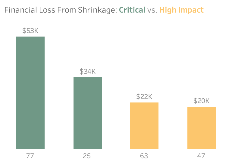
Four locations account for 65% of total annual shrinkage ($200K), split into $94K direct cost and $35K lost margin. Store 77 is the highest-risk location at $53K in exposure, likely amplified by its large SKU assortment. This concentration indicates that focusing resources on a handful of stores is likely to deliver the greatest reduction in losses.

2. Operational Leakage Dominates: Low-Value Items Drive 88% of Shrinkage Value

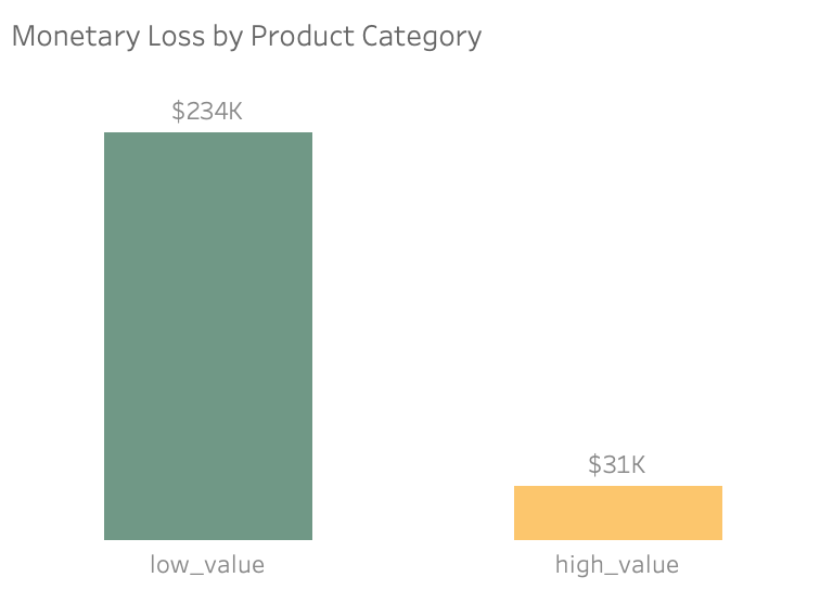
Low-value items account for 88% of total shrinkage ($233K of $264K), driven by transaction volume rather than unit price. High-value items show higher per-unit loss rates but minimal contribution to total loss. This suggests operational process failures, rather than theft of high-value items, are the primary driver of shrinkage.

3.Capital Inefficiency Represents the Largest Structural Risk: $28M Locked in Slow-Moving Inventory

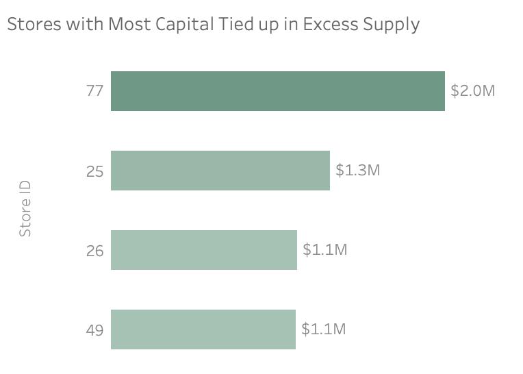
Across the network, 8,198 SKUs exceed 90 days of supply, tying up $28M in working capital. Inventory is highly concentrated — four stores (77, 26, 49, and 25) alone account for $5.5M, with Store 77 alone contributing nearly $2M.
Stores 64, 77, 40, and 49 each hold more than 700 days of inventory, indicating severe overstock and slow inventory turnover. Reducing excess inventory would improve cash flow, free working capital, and lower the risk of inventory becoming obsolete.

4. Vendor Delivery Inaccuracies Create Systemic Stock Imbalances

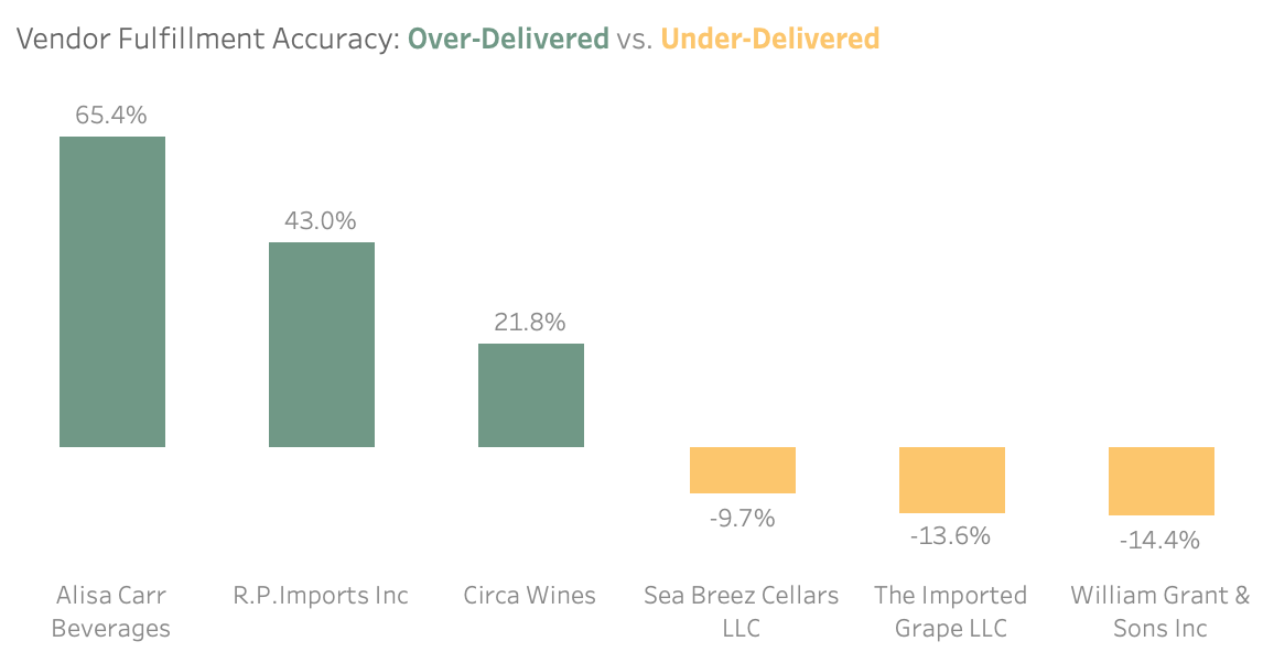
Inventory variance is concentrated among specific vendors rather than distributed randomly. William Grant & Sons Inc shows cumulative under-deliveries exceeding 35K units, while Alisa Carr Beverages over-delivered by approximately 65% relative to orders. These patterns are consistent across multiple products, indicating persistent fulfillment errors. Addressing a small number of high-variance vendors could significantly improve inventory accuracy across the network.

5. Geographic Patterns Reveal Distinct Operational Failure Modes

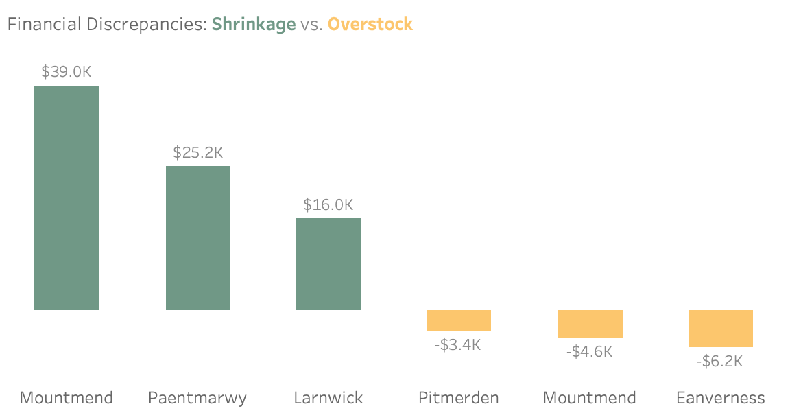
Losses cluster geographically, with Store 77 (Mountmend) and Store 25 (Paentmarwy) accounting for $64K+ in shrinkage. In contrast, Stores 49 (Eanverness) and 40 (Pitmerden) show significant overstock relative to recorded deliveries, indicating localized receiving and inventory control failures. The differing patterns across stores indicate that a single company-wide solution is unlikely to be effective; interventions should be tailored by location.

Recommendations

1. Stabilize Inventory in High-Risk Stores

Phase 1.1 — Critical Stores (Immediate Focus)

Target Stores: 77, 25, 26, 49
These stores show overlapping issues in shrinkage, excess inventory, and stock imbalance. Actions:

• Focused full inventory reconciliation for all SKUs
• Tighten receiving and stock movement controls
• Introduce frequent cycle counts for high-variance SKUs
• Temporarily restrict replenishment for items exceeding 90 days of supply

Phase 1.2 — Emerging Risk Stores

Target Stores: 63, 47, 50, 45
These stores show isolated risk signals in shrinkage or inventory imbalance, without compounding failure patterns. Actions:

• Apply Phase 1 control framework at reduced frequency
• Monitor shrinkage and days-of-supply trends continuously
• Escalate stores showing worsening trends into Phase 1.1

2. Reduce Leakage in Low-Value Items

Target Category: Low-value SKUs
Low-value items are the primary driver of shrinkage by volume. Actions:

• Strengthen receiving verification for high-volume SKUs
• Increase cycle count frequency for discrepancy-prone items
• Standardize replenishment and shelf handling processes
• Reduce breakage and misplacement through tighter operational controls

3. Improve Vendor Delivery Accuracy

Target Area: High-variance vendors (under/over delivery patterns) Vendor inconsistency is driving both stockouts and excess inventory. Actions:

• Implement vendor-level tracking (ordered vs received vs billed)
• Flag vendors exceeding variance thresholds
• Enforce stricter receiving validation for high-variance suppliers
• Introduce periodic vendor performance reviews based on delivery accuracy

Limitations & Assumptions

1. Synthetic Dataset: Data is fictional; operational context (store layout, staffing, security, cycle counts) is unavailable for deeper root-cause analysis. 2. Temporal Granularity: Data is limited to annual snapshots (Start-of-Year and End-of-Year), preventing analysis of seasonal or monthly trends. 3. Demand Assumption: Days of Supply assumes constant sales velocity and does not account for seasonality or spikes. 4. Thresholding Approach: Risk thresholds (e.g., 90-day supply, percentiles) are data-driven since no predefined business benchmarks exist.